


![图片[1]-Vlookup公式还可以这么玩,太牛了!-宇程系统站](https://ycoemxt.cn/wp-content/uploads/2026/06/5d7bc31e4420260615013651-1024x683.png)
你的Vlookup公式只会查找值,而我写的Vlookup公式却自带超链接功能,而且跳转后还会高亮颜色显示。
![图片[2]-Vlookup公式还可以这么玩,太牛了!-宇程系统站](https://ycoemxt.cn/wp-content/uploads/2026/06/95923a0f3320260615012037.gif)
来看看这个公式是怎么写的:
=HYPERLINK(“#A“&MATCH(E2,A:A,0),VLOOKUP(E2,A:B,2,0))
注:如果两个表不在同一个工作表中,在A前还要带工作表名称+!
![图片[3]-Vlookup公式还可以这么玩,太牛了!-宇程系统站](https://ycoemxt.cn/wp-content/uploads/2026/06/95923a0f3320260615012105.gif)
原来在查找的同时,用hyperlink和Match函数生成超链接,而Vlookup只负责显示查找结果。
而颜色是怎么做到的?答案是VBA事件程序+条件格式
工作表右键 – 查看属性 – 在新打开的界面右侧代码窗口选取worksheet,然后在两句代码中添加一行代码:
[g1] = Target.Row
![图片[4]-Vlookup公式还可以这么玩,太牛了!-宇程系统站](https://ycoemxt.cn/wp-content/uploads/2026/06/4ce7254a9720260615012132.gif)
然后设置条件格式
=ROW(A1)=$G$1
![图片[5]-Vlookup公式还可以这么玩,太牛了!-宇程系统站](https://ycoemxt.cn/wp-content/uploads/2026/06/7ab3b22a5120260615012150.jpg)
最后还要把文件另存为启用宏的工作簿
![图片[6]-Vlookup公式还可以这么玩,太牛了!-宇程系统站](https://ycoemxt.cn/wp-content/uploads/2026/06/3a9d726bdd20260615012207.jpg)
搞定!
THE END














暂无评论内容